Ficheru:Hamiltonian flow classical.gif
Nun ta disponible con mayor resolución.
Hamiltonian_flow_classical.gif (195 × 390 píxels, tamañu de ficheru: 172 kB, triba MIME: image/gif, animáu, 86 cuadros, 26s)
Resume
| Descripción |
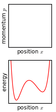
English: Flow of a statistical ensemble in the potential x**6 + 4*x**3 - 5*x**2 - 4*x. Over long times it becomes swirled up, and appears to become a smooth and stable distribution. However, this stability is an artifact of the pixelization (the actual structure is too fine to perceive). This animation is inspired by a discussion of Gibbs in his 1902 wikisource:Elementary Principles in Statistical Mechanics, Chapter XII, p. 143: "Tendency in an ensemble of isolated systems toward a state of statistical equilibrium". A quantum version of this can be found at File:Hamiltonian flow quantum.webm |
| Data | |
| Fonte | Trabayu propiu |
| Autor | Nanite |
Source
Este GIF gráfico fue creado con Matplotlib.
Esta imagen fue creada con ImageMagick.
Python source code. Requires matplotlib ImageMagick. Possibly does not run in Windows.
from pylab import *
import subprocess
import sys
import os

figformat = '.png'
seterr(divide='ignore')
rcParams['font.size'] = 9

#define color map that is transparent for low values, and dark blue for high values.
# weighted to show low probabilities well
cdic = {'red':   [(0,0,0),(1,0,0)],
        'green': [(0,0,0),(1,0,0)],
        'blue':  [(0,0.7,0.7),(1,0.7,0.7)],
        'alpha': [(0,0,0),
                  (0.1,0.4,0.4),
                  (0.2,0.6,0.6),
                  (0.4,0.8,0.8),
                  (0.6,0.9,0.9),
                  (1,1,1)]}
cm_prob = matplotlib.colors.LinearSegmentedColormap('prob',cdic,N=640)

### System dynamics ###

# potential is a polynomial
potential_coefs = array([1,0,0,4,-5,-4,0],'d')
def potential(x,t):
    return polyval(potential_coefs,x)

# force function is its derivative.
force_coefs = (potential_coefs*arange(len(potential_coefs)-1,-1,-1))[:-1]
def force(x,t):
    """ derivative of potential(x) """
    return polyval(force_coefs,x)
invmass = 1.0
dt = 0.03

def motion(t,x,p):
    """ returns dx/dt, dp/dt """
    return p*invmass, -force(x,t)

cur_x = -0.1
cur_p = 0

def rkky_step(t, x_i, p_i, dt):
    kx1,kp1 = motion(t, x_i, p_i)
    dt2 = 0.5*dt
    kx2,kp2 = motion(t+dt2, x_i+dt2*kx1, p_i+dt2*kp1)
    kx3,kp3 = motion(t+dt2, x_i+dt2*kx2, p_i+dt2*kp2)
    kx4,kp4 = motion(t+dt, x_i+dt*kx3, p_i+dt*kp3)
    newx = x_i + (dt/6.0)*(kx1 + 2.0*kx2 + 2.0*kx3 + kx4)
    newp = p_i + (dt/6.0)*(kp1 + 2.0*kp2 + 2.0*kp3 + kp4)
    return newx, newp

### Setup ensemble points ###

# most are randomly chosen
x = 0 + 0.5*rand(20000)
p = -1.0 + 2.0*rand(20000)

# the pilot points are set manually
x[0] = 0;    p[0] = 0
x[1] = 0.4;  p[1] = 0.0
pilots = [0,1]
pilot_colors = {
       0: (0,0.7,0),
       1: (0.7,0,0)}
E = potential(x,0) + 0.5*invmass*p**2

### set up plot limits and histogram bins ###
xedges = linspace(-2.1,1.7,151)
pedges = linspace(-7.5,7.5,151)
Eedges = linspace(-9,9,151)
pix = 150
extent = [xedges[0], xedges[-1], pedges[-1], pedges[0]]
H = histogram2d(x,p,bins=[xedges,pedges])[0].transpose()
cmax = amax(H)*0.8

extenten = [xedges[0], xedges[-1], Eedges[-1], Eedges[0]]
Hen = histogram2d(x,E,bins=[xedges,Eedges])[0].transpose()
cmaxen = amax(Hen)*0.3

fig = figure(1)
ysize = 2.6
xsize = 1.3
fig.set_size_inches(xsize,ysize)

### Prepare lower plot ###
axen = axes((0.2/xsize,0.2/ysize,1.0/xsize,1.0/ysize),frameon=True)
axen.xaxis.set_ticks([])
axen.xaxis.labelpad = 2
axen.yaxis.set_ticks([])
axen.yaxis.labelpad = 2
xlim(-2.1,1.7)
ylim(-9,9)
xlabel('position $x$')
ylabel('energy')
potx = linspace(-2.1,1.7,151)

### Prepare upper plot ###
ax = axes((0.2/xsize,1.5/ysize,1.0/xsize,1.0/ysize),frameon=True)
ax.xaxis.set_ticks([])
ax.xaxis.labelpad = 2
ax.yaxis.set_ticks([])
ax.yaxis.labelpad = 2
xlim(-2.1,1.7)
ylim(-7.5,7.5)
xlabel('position $x$')
ylabel('momentum $p$')

### Start running simulation ###
frames = list()
delays = list()
framemod = 5
frame = "frames/background"+figformat
savefig(frame,dpi=pix)
frames.append(frame)
delays.append(16)

print "generating frames...  0%",
sys.stdout.flush()
savesteps = range(0,401,framemod) + [600, 1000, 2000, 6000]
delays += [10]*len(savesteps)
delays[1] = 200
delays[-5:] = [100,200,200,200,400]
totalsteps = max(savesteps)+1
for step in range(totalsteps):
    if step % 20 == 0:
        print "\b\b\b\b\b{0:3}%".format(int(round(step*100.0/totalsteps))),
        sys.stdout.flush()
    if step in savesteps:
        # Every several frames, do a plot
        remlist = list()

        sca(ax)
        H = histogram2d(x,p,bins=[xedges,pedges])[0].transpose()
        remlist.append(imshow(H, extent=extent, cmap=cm_prob, interpolation='none', aspect='auto'))
        remlist[-1].set_clim(0,cmax)
        for i in pilots:
            remlist += plot(x[i], p[i], '.', color=pilot_colors[i], markersize=3)

        E = potential(x,step*dt) + 0.5*invmass*p**2
        sca(axen)
        pot = potential(potx,step*dt)
        remlist += plot(potx,pot,color='r',zorder=0)
        Hen = histogram2d(x,E,bins=[xedges,Eedges])[0].transpose()
        remlist.append(imshow(Hen, extent=extenten, cmap=cm_prob, interpolation='none', aspect='auto',zorder=1))
        remlist[-1].set_clim(0,cmaxen)
        for i in pilots:
            remlist += plot(x[i], E[i], '.', color=pilot_colors[i], markersize=3)

        frame = "frames/frame"+str(step)+figformat
        savefig(frame,dpi=pix)
        frames.append(frame)
        # Clear out updated stuff.
        for r in remlist: r.remove()
    x, p = rkky_step(step*dt, x, p,dt)
print "\b\b\b\b\b      done"

assert(len(delays) == len(frames))

### Assemble animation using ImageMagick ###
calllist = 'convert -dispose Background'.split()
for delay,frame in zip(delays,frames):
    calllist += ['-delay',str(delay)]
    calllist += [frame]
calllist += '-loop 0 -layers Optimize _animation.gif'.split()
f = open('anim_command.txt','w')
f.write(' '.join(calllist)+'\n')
f.close()

print "composing into animated gif...",
sys.stdout.flush()
subprocess.call(calllist)
print "      done"
os.rename('_animation.gif','animation.gif')
Llicencia
Yo, el titular de los drechos d'autor d'esta obra, la espublizo baxo la siguiente llicencia:
| Esti ficheru ta disponible baxo la llicencia Creative Commons de Dedicatoria universal al dominiu públicu CC0 1.0. | |
| La persona qu'asoció una obra con esti documentu dedicó esa obra al dominiu públicu per aciu de la cesión mundial de los sos drechos baxo les lleis de drechos d'autor, incluyendo tolos los drechos llegales rellacionaos y axacentes, dientro del ámbitu permitíu pola llei. Pue copiar, camudar, distribuir y reproducir la obra, incluyendo con oxetivos comerciales, ensin pidir permisu.
|
Historial del ficheru
Calca nuna fecha/hora pa ver el ficheru como taba daquella.
| Data/Hora | Miniatura | Dimensiones | Usuariu | Comentariu | |
|---|---|---|---|---|---|
| actual | 08:57 27 och 2013 | | 195 × 390 (172 kB) | Nanite | Added potential plot (with bonus ensemble histogram in E,x), as well as a couple of "pilot" systems. |
| 22:39 26 och 2013 |  | 195 × 195 (84 kB) | Nanite | higher resolution + a big longer in time to get the smooth look. | |
| 22:10 26 och 2013 |  | 195 × 195 (84 kB) | Nanite | User created page with UploadWizard |
Usu del ficheru
La páxina siguiente usa esti ficheru:
Usu global del ficheru
Estes otres wikis usen esti ficheru:
- Usu en ar.wikipedia.org
- Usu en az.wikipedia.org
- Usu en en.wikipedia.org
- Usu en en.wikiversity.org
- Usu en es.wikipedia.org
- Usu en fr.wikipedia.org
- Usu en id.wikipedia.org
- Usu en ja.wikipedia.org
- Usu en pt.wikipedia.org
- Usu en sl.wikipedia.org